Projects

  • Tablet Dissolution Analysis

    Zoetis intern project using Databricks to integrate Neo4j, Azure, Ignition, and Power BI data and analyze which manufacturing factors most influence final product dissolution rate.

    This analysis was done as a Data Science Intern for Zoetis in the summer of 2026. Because the data is proprietary, I’ll give only a rough overview.

    Goal

    At the end of its manufacturing process, a certain drug undergoes various tests to verify that it was made correctly and is ready to be sold. Because the drug is administered orally, as a tablet, one of the tests is a dissolution test: you take a sample of the tablets, put them in water under controlled conditions, and measure the amount of each active ingredient dissolved at certain time points. If the average rate of dissolution falls within the approved range, the batch passes, and if not, it fails and must be retested or discarded.

    Zoetis had years of data about this product, covering periods when it passed all its dissolution tests, periods when it often failed, and various combinations of vendors and recipes of the ingredients. My task was to perform a multivariate analysis to tease out the most likely underlying causes of weaker dissolution test results. Do batches using ingredient A bought from vendor 3 perform worse than when A is bought from vendor 1 or vendor 2? Does some attribute of ingredient B, like pH or granule size or percentage of loss on drying, correspond to faster dissolution? Does running the tablet press with greater level of force result in more compact and thus slower-dissolving tablets? The possible causes are basically limitless, but if we could identify the factors that have the biggest influence on dissolution and tighten our control of those parameters, we could reduce the money and time spent retesting and discarding failed batches.

    Data Preparation

    I pulled data from four sources:

    • A SQL Server database holding continued process verification and lab testing data
    • A Neo4j graph database holding manufacturing genealogy data
    • A table in Azure holding manufacturing equipment data collected by Ignition and preprocessed in Databricks
    • A PowerBI dashboard displaying dissolution stage testing results for the product

    It was all rather complicated—having to resolve column name discrepancies; identify and correct likely misinputs; merge columns representing the same attribute measured on different variants of the same material; figure out why some attributes were so often null and whether this was expected or problematic; decide the best definition of a dissolution “failure” (failed stage 1? failed any stage? was discarded?); write a Cypher query that handled arbitrarily long chains of a batch being a component of itself; take the weighted mean of each attribute when different batches of an ingredient having different attribute values are used in a single batch of the final product; create meaningful batch-level features from Ignition time series data; engineer a response variable allowing dissolution tests of different active ingredients, time points, and tablet sizes to be fairly compared to one another; determine whether to incorporate or remove tests flagged in PAS-X and non-standard inspection types; and more. When all was said and done, 80% of the project was understanding, querying and cleaning the data, deriving useful features from it, and combining it into a table fit for machine learning.

    Analysis

    Using MLflow in Databricks, I trained and tracked a few dozen models to predict the results of the dissolution tests of a batch based on the variant (one-hot encoded) and attributes (quantitative) of each ingredient and the Ignition equipment data. I used machine learning best practices—feature selection, cross-validation, standardization, grid search over hyperparameter combinations, etc.

    The two strongest predictors—both XGBoost regressors, trained to predict two different representations of the underlying dissolution data—each gave the highest permutation scores to the same two features: the use of a particular vendor of one ingredient, and the value of a particular attribute of another. A few other factors had weaker, but not insignificant, effects.

    I presented my results to the head of the plant where the product is manufactured, and she assigned a lab tech to design a study to determine whether the results were causal and, if so, how best to control them moving forward.

    I also delivered an impact-focused presentation of my results to an assembly of business leaders, including the Chief Digital and Technology Officer.

  • Semantic Tuple Diversification

    Designed and built a system that finds tables in a data lake that can be joined to a user-provided table and suggests string columns to add based on their semantic difference from the user’s table.

    I undertook this project with two of my classmates under the direction of Dr. El Kindi Rezig of the Kahlert School of Computing at the University of Utah, whose research often focuses on algorithmic solutions to the messy, tedious of data engineering, such as data discovery, data integration, and the management of large-scale data lakes. Our goal was to build a system to address the following scenario: a user has a table with information of interest to her, she would like to expand it by adding more columns, and she must find these columns amid a data lake of tables with inconsistent schemas. In addition, she would like to ensure the columns she adds bring in as much new information as possible, so the system must measure semantic, not merely syntactic, differences between strings.

    Our system identifies plausible joins, builds a join graph, identifies string columns from the joinable tables, quantifies how much semantic diversity (meaningful new information) each candidate string column would add to the existing dataset, and ranks candidate columns from most to least diversity added. In short, it surfaces columns from the lake most likely to give the user new information about the entities in his table.

    My contribution to the project code was the join graph builder, which was challenging in its own right but was only the initial requirement for solving our overarching goal. I did not write any code for embedding columns, quantifying diversity, ranking the columns. However, each step was a cooperative creative process; I spent about 20 hours with my teammates throughout the semester discussing theory and pseudocode about how to solve these problems, during which I contributed several of the key ideas that led to our solution. I also went through all the project code in detail with my teammates when were finished, so even though I didn’t write all of it, I have a thorough understanding of the finished system.

    See a demonstration of the system and our complete report below.
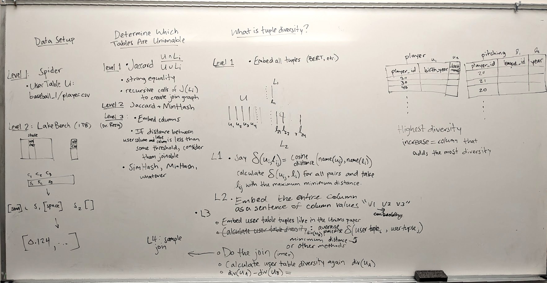
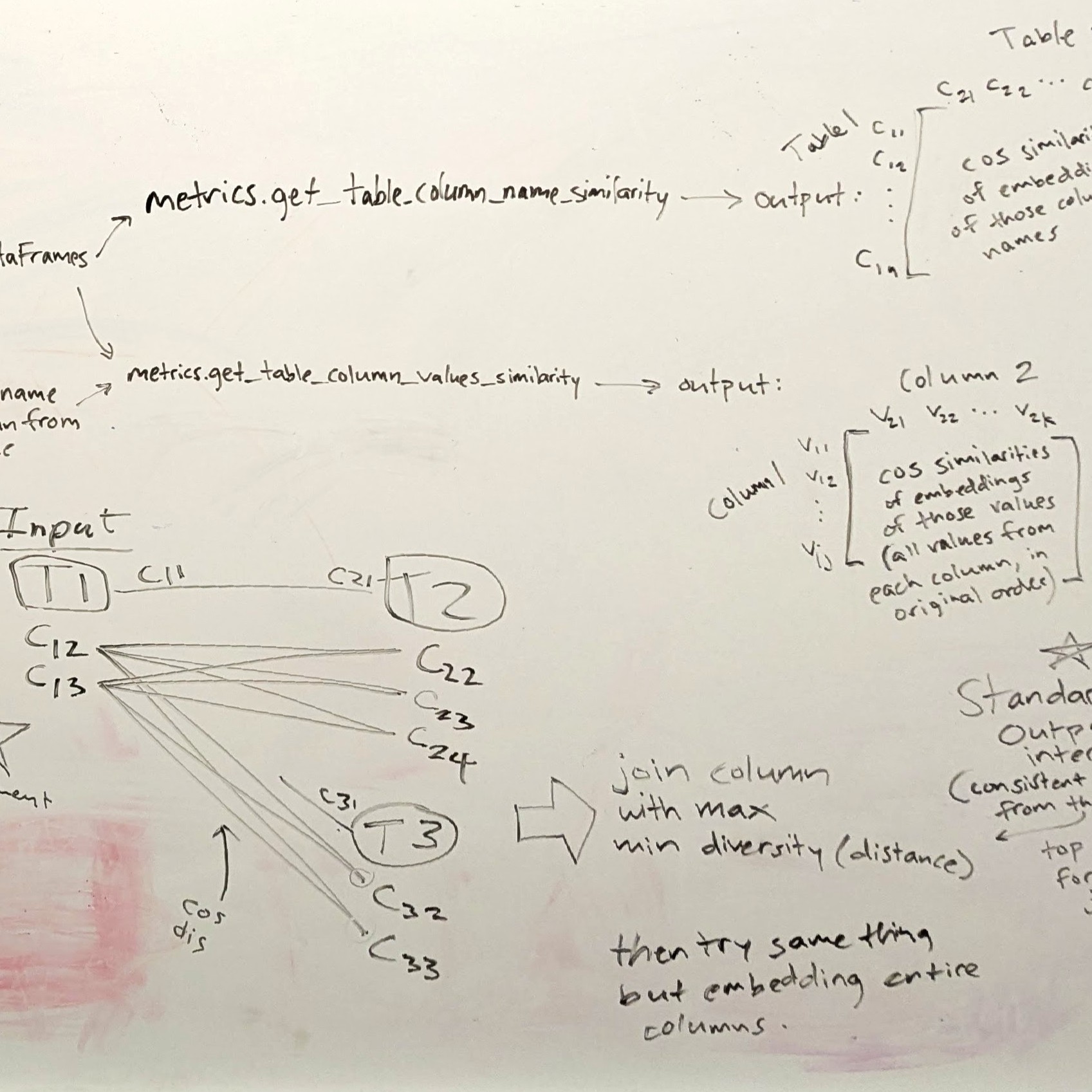
    The result of our first brainstorming session—our first attempt to outline a complete solution (handwriting mine)

    Demonstration

    Final report

  • Drive for Show, Putt for Dough

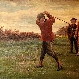
    How accurate is the famous saying?     (a web app using Flask and Plotly)                     

  • Clustering Medical Conditions by Prescribed Drug

    Exploring relationships between medical conditions and the drugs prescribed for them using data from the 2023 Medical Expenditure Panel Survey.

    Data Processing

    1) By joining the MEPS Medical Conditions file (COND) and the Prescribed Medicines file (RX) via the Condition-Event Link file (CLNK), we created a dataset where each row was a prescription event: one instance of a person filling or refilling a drug, including the name of the drug and for what condition it was prescribed. (281,158 rows, 11 variables.)

    2) After removing refills (so each patient–drug–condition combination was counted only once), removing rare conditions and drugs (<25 occurrences), and aggregating the drugs into 16 therapeutic classes, we created a condition–drug co-occurrence matrix: each of the 206 rows was a condition, each of the 16 columns was a drug class, and each cell held the number of times they occurred together in a prescription event. This matrix answers the question, “How many people in the sample were ever prescribed a drug in class D for condition C?”
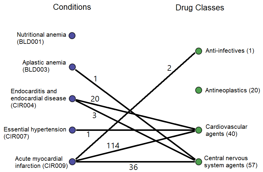
    Conceptually, this matrix represents a bipartite graph connecting conditions to the classes of drugs prescribed for them, with edge weights equaling the number of people to whom such a prescription was given. That graph would look like this, but with 201 more conditions and 12 more drug classes (the weights are from the real data).
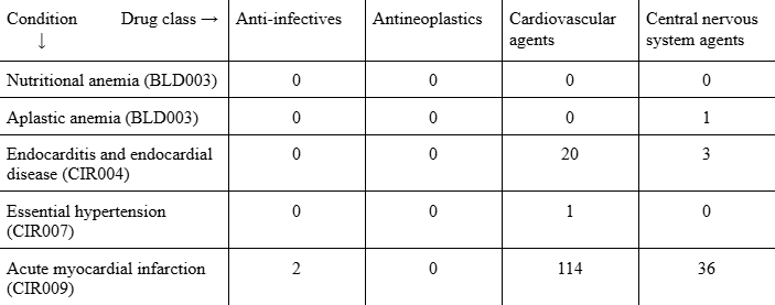
    Literally, the matrix looks like this (with 12 more columns and 201 more rows).
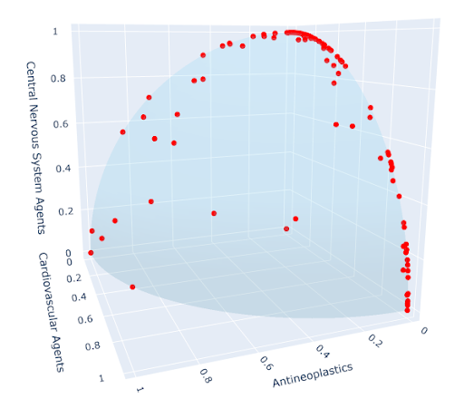
    3) Since we were interested only in which drugs were typically prescribed for each condition, not how often the conditions occurred, we performed a final step: normalization. After normalization, each vector has an L2 norm of 1, so the data can be visualized as points on the unit sphere in 16 dimensions, all lying in the positive orthant or on an axis bordering it. Using only the first three dimensions, we get the figure at left; try to envision the impossible, an analogous figure in 16 dimensions, and you’ll have a good understanding of the final data structure.

    The higher the value of a coordinate, the more often drugs of that class are prescribed for that condition.

    Clustering

    We used three clustering methods:

    • K-means
    • Hiearchical agglomerative clustering (HAC)
    • Mixture of von Mises–Fisher distributions (vMF) (I was responsible for this model, which I borrowed from Banerjee, Arindam; Dhillon, Inderjit S.; Ghosh, Joydeep; Sra, Suvrit (2005). Clustering on the Unit Hypersphere using von Mises-Fisher Distributions. Journal of Machine Learning Research, 6, 1345–1382.)
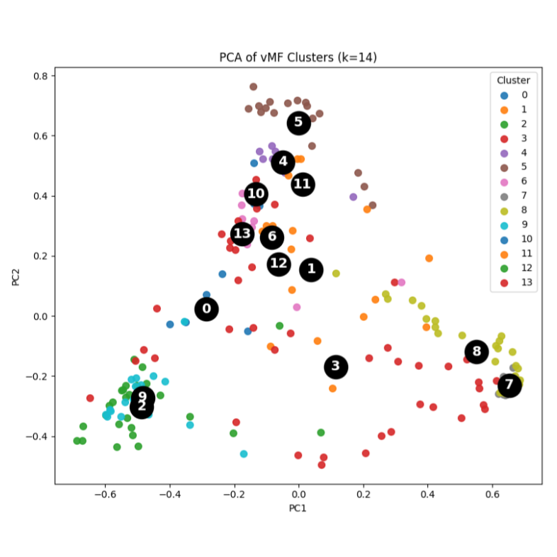
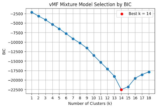
    Using BIC, the optimal number of clusters was 14 (click to show plot).
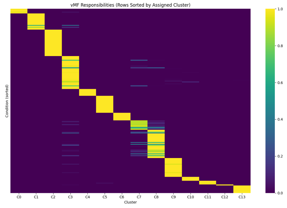
    The soft cluster assignments were mostly confident, but there is some uncertainty about the boundaries between a few of the clusters, most notably 3, 7, and 8 (click to show plot; the lighter the color, the higher likelihood the point represented by the row belongs to the cluster represented by the column).
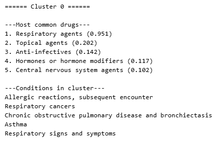
    At right (or below, on mobile) is an example cluster. For each cluster, we found the mean vector—the “characteristic condition” of that cluster—and used it to identify the cluster’s typical prescription pattern. The number in parentheses is the coordinate, representing how frequently the drug class is prescribed for conditions in the cluster. (Keep in mind the coordinates don’t have a meaningful unit; the most specific valid interpretation is “higher means more frequent.”)
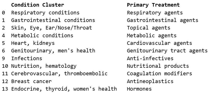
    All three methods produced similar clusters with similar themes. We identified cluster themes manually by looking at the types of conditions in them and the types of drugs most germane to it, then we had an LLM do the same exercise to verify our conclusions. These, roughly, were the cluster themes (the numbers are arbitrary, just identifiers):
    Click here to see the complete set of clusters.

    Takeaways

    Most of the analysis validates common-sense conclusions. Of course most respiratory conditions are treated similarly, predominantly with respiratory agents; of course most gastrointestinal conditions are treated similarly, predominantly with gastrointestinal agents; etc. Where clusters are clean, no questions are raised.

    Three of the clusters are less clear. To me, these are the interesting ones. I’ll conclude with a few potential questions:

    The division between cluster 7, which we’ve informally labeled as “central nervous system (CNS) disorders,” and cluster 8, which we’ve called “mental health conditions,” is blurry. (In fact, k-means and HAC didn’t even make them distinct clusters.) Cluster 7 is treated almost exclusively by CNS agents, while cluster 8 is treated primarily by CNS agents but also has a very common secondary drug class: psychotherapeutic agents. Why are these clusters so intertwined? It would be satisfying if, waiting to be unearthed here, there were two clusters with different primary drug classes: one for conditions best treated by CNS agents, and one for conditions best treated by psychotherapeutic agents. Can further study of these conditions reduce the variation in how cluster 8 is treated, leading to the emergence of two distinct groups?

    Cluster 3 is the largest, has the largest variety in prescriptions, and has many low-confidence assignments. K-means and HAC both produced a similar cluster. This cluster is a sort of mixed bag: no strong unifying type of condition, no strong unifying treatment. Every condition in this cluster, then, raises questions of its own. If there isn’t a consistently applied treatment method, it implies a strong, effective treatment method isn’t known (or else it would be used consistently); can one be discovered? Or, if a condition in this cluster does have a consistent treatment, then it’s categorized here because there are few or no similar conditions, begging the question “what makes that condition so unusual?”

  • Android Malware Classification Pipeline

    A Scikit-learn data transformation and model training pipeline comparing the effectiveness of four machine learning models on a classification task with sparse data.

    This is a brief overview of the machine learning workflow I built to classify Android software as “malware” or “not malware” for a Kaggle competition which served as the final project for my graduate-level machine learning course. Full implementation details are found in the report below and the linked GitHub repository.

    Data Loading and Setup

    First I imported training and testing datasets and calculated basic descriptive statistics: 3,124 training examples, 241 sparse numeric features, and notable class imbalance (79.8% belonging to the majority class). I established a fixed random seed (67) to ensure reproducible results.

    Train–Validation Split

    Before any modeling, I split the data 80/20. 80% was used to train the model; the remaining 20% was a dedicated validation set that never entered the cross-validation folds, letting it act as the final test for models before they were delivered as Kaggle submissions.

    Establishing a Baseline

    To set a minimum performance standard, I tested two simple classifiers: a majority-class classifier (always selects the majority class) and a stratified random classifier (selects a class at random with each class weighted by the proportion of the data it comprises). These established the macro-F1 score floor that any useful machine learning model needed to beat.

    Learning Pipeline Construction

    A reusable automated pipeline was built using the imblearn library to ensure every data transformation was performed correctly during cross-validation. The pipeline included four stages:

    • Imputation: Using the Impyute library to fill missing values with column means.
    • Scaling: Applying StandardScaler to normalize numeric features.
    • Resampling: Using synthetic minority over-sampling technique (SMOTE) to address class imbalance (or passing through without changes).
    • Classification: Inserting the machine learning algorithm to be tested.

    Grid Search and Cross-Validation

    I tuned the model hyperparameters using GridSearchCV (or RandomSearchCV for models with more hyperparameter options) with stratified 5-fold cross-validation, optimizing for macro-F1 score.

    Model Implementation and Comparison

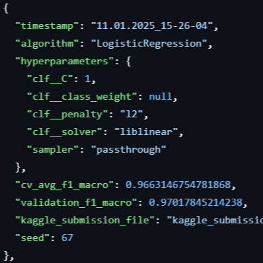
    I tried four different machine learning algorithms (logistic regression, linear support vector machine, random forest, and XGBoost) and compared the results. Frankly, they all performed about the same (F1 scores in the range 0.97 ± 0.5):

    Evaluation and Logging

    At the start of the project, I implemented a detailed logging system to track each experiment’s parameters, CV scores, and timestamps, ensuring the methodology and results remained organized and transparent. The key takeaway of the project was that although the results were similar for each model, the results of my earlier attempts (before I had implemented a thorough data transformation pipeline) were significantly worse, so it appears that preparing the data properly is more significant (at least in this case) than the particular model you use. Also, though the models were equal in results, they were very unequal in training time, which makes a strong case for using simple models whenever possible and ramping up to more complex models, which can take orders of magnitude longer to train, only if necessary.

    Full Report

  • Knot Invariants Research Using Supervised Learning

    Created a custom encoding for the Jones polynomial and used it to predict other knot invariants with the Keras Sequential API.

    As a junior at BYU, I was hired by a research group in the mathematics department headed by Dr. Mark Hughes, who specializes in low-dimensional topology, including knot theory. Knot theory involves more data than most areas of pure mathematics research—a theoretically infinite number of knots, thousands of which have been characterized and catalogued, each described by dozens of mathematical attributes (“invariants”)—so he created the research group to explore data-oriented approaches to the study of knots.

    The question that came to occupy most of my time was this: could machine learning uncover unexpected interactions among knot features? In other words, could it identify large-scale patterns in knot invariants that, according to known theory, should not be there? If so, it would hint at latent mathematical structure that topologists could then investigate.

    I used KnotInfo1, a database of all 12,965 prime knots with crossing number up to 13 and all their known invariants.2 (A prime knot is one that isn’t made by connecting two smaller prime knots; the crossing number is the minimum number of crossings in any diagram of the knot). Most invariants are known for lower-crossing knots, but as the number of crossings grows, so does the difficulty of calculating invariants; thus, not every knot in the database has a value for every invariant. But there’s enough to work with. I also used Matlab code Dr. Hughes had previously written to pseudo-randomly generate knots of arbitrary crossing number, so our dataset could include knots larger than crossing number 13.
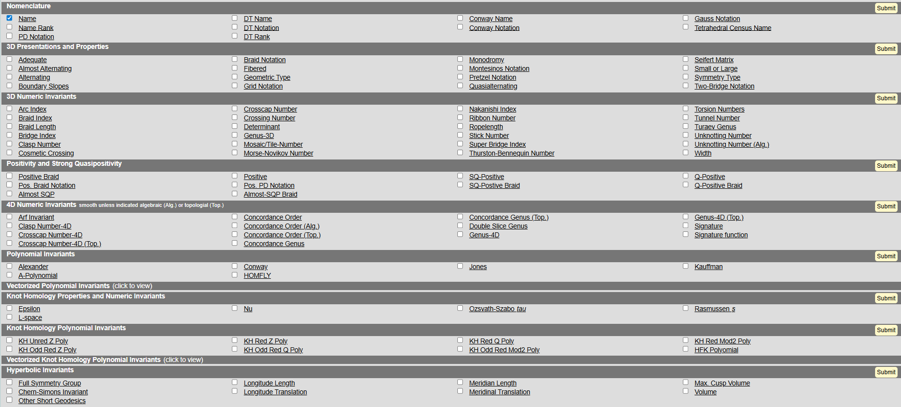
    All invariants included (if known) for each knot in the KnotInfo database

    Here are the details for the approach that proved successful (meaning that among a lot of predictable, boring results I found a single unpredictable, interesting one). I set out to see if I could accurately predict any of a knot’s invariants using only its Jones polynomial.

    Data Validation

    First I filtered out knots for which the Jones polynomial was not definitively known—in KnotInfo, where the lower bound did not equal the upper bound, or in the generated dataset, where the Jones calculation returned “failed.”

    Encoding the Features

    Example Jones polynomial: V(t)=t3+3t23t1+33t+2t2t3V(t) = -t^{-3}+3t^{-2}-3t^{-1}+3-3t+2t^2-t^3

    Since Jones polynomials are strings, I had to parse them into a format machine learning models could accept. I wrote a custom parser to turn them into lists where the index corresponds to the exponent, in the order 0, 1, -1, 2, -2, …, and the value is the coefficient. The example above would have become [3, -3, -3, 2, 3, -1, -1]. Each list index becomes its own feature column.

    Different knots have different Jones polynomial lengths, so I padded the end of each list, appending zeros until each was as long as the longest list in the dataset. Generally, filling missing values with zeros would be bad practice, but in this case it is an appropriate solution; each list element represents the coefficient of one term in a polynomial, so a list element being nonexistent is mathematically equivalent to it being zero (e.g., x^2 = x^2 + 0x + 0). This made the inputs consistent and ready to input into a neural net.

    Model Setup

    Since I wanted to predict as many invariants as possible using only the Jones polynomial, I made it so I could pass in the name of an invariant and a model would train using Jones as the input and the named invariant as the target. This was a baseline framework I would have expanded had I stayed with the research group longer; every invariant, some with various possible encodings, could have been either an input or an output of this generalized model pipeline, and I then I could have compared every 1:1 input:output combination, or which combinations of invariants were more predictive than any one alone.

    I first used Jones to predict all the integer invariants, since those were the easiest to encode; you can either treat them as numbers or treat them as categories using a label encoder, and both are simple to set up. My model architecture was a simple neural network using the Keras API over TensorFlow, trained independently for each target invariant. These were my prediction accuracies on each test set:
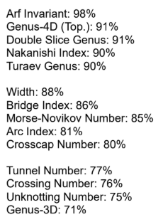
    From here, my ability to contribute was nil; I had no training in topology, so I didn’t know what any of these invariants were or whether evidence of their connection to the Jones polynomial was significant. I emailed the results to Dr. Hughes’s, who said the connection between the Jones polynomial and the Arf invariant was well known, but the result for Genus-4D was a little more suprising. Additionally, he later discovered a bug in his Matlab code that was causing it to produce invalid knots, and once it was fixed, the accuracy of 4D genus predictions jumped even higher, to 97.7%.

    Unfortunately, I left the research group soon afterward, but Dr. Hughes told me it continued to be a significant research question for him for some time. A group of physicists in South Africa he worked with expressed interest in the connection with the 4D genus, and he sent my results on to them for further testing. Meanwhile, I got a new job, and I lost the trail of the research. But it was fun while it lasted!

    Code

    import sys
    import numpy as np
    import os
    import pandas as pd
    import math
    import datetime
    import random
    from sklearn.model_selection import train_test_split
    import tensorflow as tf
    
    pd.set_option('display.max_columns', None)
    pd.set_option('display.expand_frame_repr', False)
    pd.set_option('max_colwidth', None)
    generated_knots = pd.read_csv('Train 1.txt')
    knots_for_training = pd.read_csv('Database Knots.csv')    # Knots from database
    og_knots_for_predicting = pd.read_csv('Predict 1.txt')    # For making predictions
    def GetOneJonesList(generatedJones):
        temp = generatedJones.replace('[','').split('],')
        temp[-1] = temp[-1].replace(']','')
        for i in range(len(temp)):
            temp[i] = temp[i].split(',')
            temp[i][0], temp[i][1] = int(temp[i][0]), int(temp[i][1])
        
        newJones = []
        n = 0
        while n <= max( abs(temp[0][0]), temp[-1][0] ):
            zero = True
            for i in temp:
                if i[0] == n:
                    newJones.append(i[1])
                    zero = False
            if zero:
                newJones.append(0)
            if n > 0:
                n *= -1
            else:
                n -= 1
                n *= -1
        return newJones
    
    def GetInvariantLists(generated_knots, other_invariant):
        if other_invariant == 'Genus-4D':
            other_invariant = 'Slice genus lower bound'
        
        cleaned_dataframe = generated_knots[~generated_knots['Jones Polynomial'].str.contains('Failed')]
        cleaned_dataframe = cleaned_dataframe[generated_knots['Slice genus lower bound'] == generated_knots['Slice genus upper bound']]
        
        jonesLists = list(cleaned_dataframe['Jones Polynomial'])
        otherList = list(cleaned_dataframe[other_invariant])
        
        newJonesLists = []
        for i in jonesLists:
            newJonesLists.append(GetOneJonesList(i))
        return newJonesLists, otherList
    
    def GetNumber(jones, j):
        number = ''
        while j < len(jones) and jones[j].isdigit():
            number += str(jones[j])
            j += 1
        return int(number), j
    
    def GetExponent(jones, j):
        if j >= len(jones) or jones[j] != '^':
            return 1
        else:
            exponent = 0
            if jones[j+1].isdigit():
                exponent, useless = GetNumber(jones, j+1)
            elif jones[j+1] == '(':
                positiveExponent, useless = GetNumber(jones, j+3)
                exponent = positiveExponent * -1
            return exponent
    
    def ProcessSegment(jones, i):
        position = 0
        if jones[i+1] == 't':
            if i == -1:
                value = 1
            elif jones[i] == '+':
                value = 1
            else:
                value = -1
            
            if i+2 >= len(jones):
                position = 1
            else:
                position = GetExponent(jones, i+2)
        elif jones[i+1].isdigit():
            value, nextIndex = GetNumber(jones, i+1)
            if jones[i] == '-':
                value = value * -1
            if nextIndex >= len(jones) or jones[nextIndex] == '+' or jones[nextIndex] == '-':
                position = 0
            elif jones[nextIndex] == '*':
                position = GetExponent(jones, nextIndex + 2)
        return position, value
    
    def GetJonesDictionary(jones):
        jonesDictionary = {}
        if (jones[0] == 't') or jones[0].isdigit():
            position, value = ProcessSegment(jones, -1)
            jonesDictionary[position] = value
        for i in range(len(jones)):
            if (jones[i]=='+' or (jones[i]=='-' and jones[i-1]!='(')):
                position, value = ProcessSegment(jones, i)
                jonesDictionary[position] = value
        return jonesDictionary
    
    def GetJonesList(jones):
        jonesDictionary = GetJonesDictionary(jones)
        powers = list(jonesDictionary.keys())
        radius = max(abs(min(powers)), abs(max(powers)))
        
        jonesList = []
        jonesList.append(jonesDictionary.get(0, 0))
        
        for i in range(1, radius+1):
            jonesList.append(jonesDictionary.get(i, 0))
            jonesList.append(jonesDictionary.get(-i, 0))
        return jonesList
    
    def ReformatJonesPolynomials(knots):
        multiJonesList = []
        generated = 'Jones Polynomial' in knots.columns
        
        if not generated:
            for i in knots.index:
                jones = knots['Jones'][i]
                multiJonesList.append(GetJonesList(jones))
        else:
            multiJonesList, useless = GetInvariantLists(knots, 'Genus-4D')
        return multiJonesList
    def GetIndicesToRemove(knots, columnTitle):
        indices = []
        invariants = list(knots[columnTitle])
        for i, inv in enumerate(invariants):
            if isinstance(inv, (int, float)):
                if math.isnan(inv): indices.append(i)
            elif isinstance(inv, str):
                if not inv.isdigit(): indices.append(i)
        return indices
    
    def ShuffleLists(joneses, other):
        c = list(zip(joneses, other))
        random.shuffle(c)
        return zip(*c)
    
    def FilterTerms(joneses, jones_terms):
        longestJones = len(max(joneses, key=len))
        newJoneses = []
        for jones in joneses:
            newJones, n = [], 0
            for index in range(longestJones):
                val = jones[index] if index < len(jones) else 0
                if n in jones_terms:
                    newJones.append(val)
                n = (n - 1) * -1 if n <= 0 else n * -1
            newJoneses.append(newJones) 
        return newJoneses
    
    def ListPrep(generated_knots, Indiana_database_knots, nonJonesInvariant, jones_terms, shuffle, test_split):
        badIndices = GetIndicesToRemove(Indiana_database_knots, nonJonesInvariant)
        joneses = ReformatJonesPolynomials(Indiana_database_knots)
        other = list(Indiana_database_knots[nonJonesInvariant])
        
        for i in reversed(badIndices):
            joneses.pop(i)
            other.pop(i)
        other = list(map(int, other))
    
        if not generated_knots.empty:
            gen_jones, gen_other = GetInvariantLists(generated_knots, nonJonesInvariant)
            joneses.extend(gen_jones)
            other.extend(gen_other)
    
        if shuffle:
            joneses, other = ShuffleLists(joneses, other)
        if jones_terms:
            joneses = FilterTerms(joneses, jones_terms)
        
        if test_split:
            return train_test_split(joneses, other, test_size=test_split)
        return joneses, other
    
    def PadTensors(t1, t2):
        s1, s2 = t1.shape[1], t2.shape[1]
        if s1 > s2:
            t2 = tf.pad(t2, [[0,0], [0, s1-s2]], 'CONSTANT')
        elif s1 < s2:
            t1 = tf.pad(t1, [[0,0], [0, s2-s1]], 'CONSTANT')
        return t1, t2
    
    def GetInputTensors(generated_knots, Indiana_database_knots, nonJonesInvariant, jones_terms=[], shuffle=True, one_hot=True, test_split=0.2):
        if test_split:
            jTrain, jTest, oTrain, oTest = ListPrep(generated_knots, Indiana_database_knots, nonJonesInvariant, jones_terms, shuffle, test_split)
            jTrain = tf.ragged.constant(jTrain).to_tensor()
            jTest = tf.ragged.constant(jTest).to_tensor()
            jTrain, jTest = PadTensors(jTrain, jTest)
            
            if one_hot:
                numOutputs = int(tf.math.reduce_max(oTrain) + 1)
                oTrain = tf.one_hot(oTrain, depth=numOutputs)
                oTest = tf.one_hot(oTest, depth=numOutputs)
            return jTrain, jTest, oTrain, oTest
        else:
            jones, other = ListPrep(generated_knots, Indiana_database_knots, nonJonesInvariant, jones_terms, shuffle, test_split)
            jones = tf.ragged.constant(jones).to_tensor()
            if one_hot:
                numOutputs = int(tf.math.reduce_max(other) + 1)
                other = tf.one_hot(other, depth=numOutputs)
            return jones, other
    
    def GetPredictionTensors(to_predict, jonesTrain, jones_terms=[]):
        to_predict = ReformatJonesPolynomials(to_predict)
        if jones_terms:
            to_predict = FilterTerms(to_predict, jones_terms)
        else:
            to_predict = tf.ragged.constant(to_predict).to_tensor()
            to_predict, _ = PadTensors(to_predict, jonesTrain)
        return to_predict
    def TrainAndEvaluateModel(generated_knots, knots_for_training, knots_for_predicting, invariant_name, jones_terms, test_split, optimizer_function, loss_function, metrics, epochs, batch_size, verbose, predict):
        tensors = GetInputTensors(generated_knots, knots_for_training, invariant_name, jones_terms, True, True, test_split)
        
        if test_split:
            jTrain, jTest, oTrain, oTest = tensors
        else:
            jTrain, oTrain = tensors
    
        if predict:
            knots_for_predicting = GetPredictionTensors(knots_for_predicting, jTrain, jones_terms)
    
        input_shape = jTrain.shape[1]
        output_shape = oTrain.shape[1]
    
        model = tf.keras.Sequential([
            tf.keras.layers.InputLayer(input_shape=(input_shape,)),
            tf.keras.layers.Dense(30, activation="softplus"),
            tf.keras.layers.Dense(30, activation="softsign"),
            tf.keras.layers.Dense(20, activation="tanh"),
            tf.keras.layers.Dense(10, activation="selu"),
            tf.keras.layers.Dense(10, activation="elu"),
            tf.keras.layers.Dense(output_shape, activation="softmax")
        ])
        
        model.compile(optimizer=optimizer_function, loss=loss_function, metrics=[metrics])
        model.fit(jTrain, oTrain, epochs=epochs, batch_size=batch_size, verbose=verbose)
        
        if test_split:
            model.evaluate(jTest, oTest)
    
        return model, knots_for_predicting
    1. C. Livingston and A. H. Moore, KnotInfo: Table of Knot Invariants, knotinfo.org, 1 Jan 2022. ↩︎
    2. I’m not going to keep track of updates to the database, so it may have changed since I was working on this project. This is just a description of what the database included at the time. ↩︎